PySpark Machine Lerning 初始化SparkSession 1 2 3 4 5 6 7 from pyspark.sql import SparkSessionspark = SparkSession \ .builder \ .appName("Python Spark Machine Lerning basic example" ) \ .config("spark.some.config.option" , "some-value" ).master("local[*]" ) \ .getOrCreate()
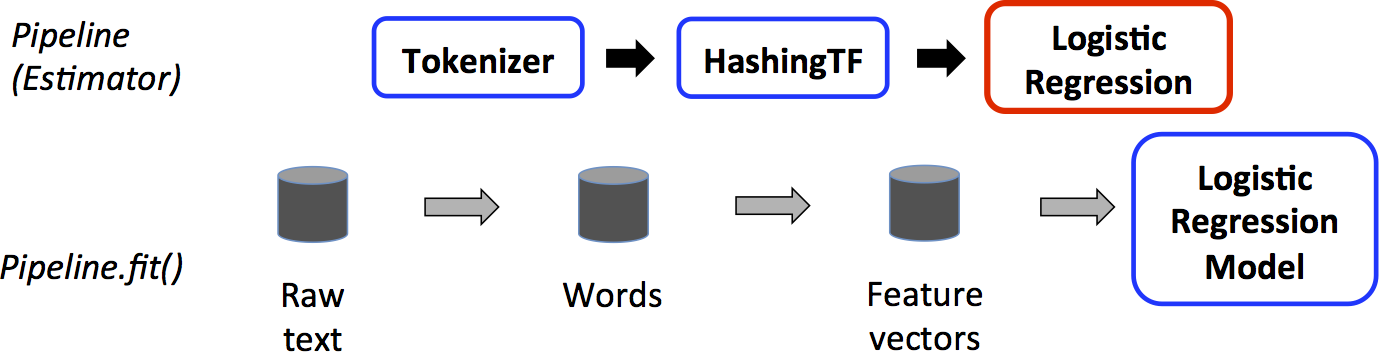
管道
1 2 3 4 5 6 7 8 9 10 11 12 13 14 15 16 17 18 19 20 21 22 23 24 25 26 27 28 29 30 31 32 33 34 35 36 37 38 39 from pyspark.ml import Pipelinefrom pyspark.ml.classification import LogisticRegressionfrom pyspark.ml.feature import HashingTF, Tokenizertraining = spark.createDataFrame([ (0 , "a b c d e spark" , 1.0 ), (1 , "b d" , 0.0 ), (2 , "spark f g h" , 1.0 ), (3 , "hadoop mapreduce" , 0.0 ) ], ["id" , "text" , "label" ]) tokenizer = Tokenizer(inputCol="text" , outputCol="words" ) hashingTF = HashingTF(inputCol=tokenizer.getOutputCol(), outputCol="features" ) lr = LogisticRegression(maxIter=10 , regParam=0.001 ) pipeline = Pipeline(stages=[tokenizer, hashingTF, lr]) model = pipeline.fit(training) test = spark.createDataFrame([ (4 , "spark i j k" ), (5 , "l m n" ), (6 , "spark hadoop spark" ), (7 , "apache hadoop" ) ], ["id" , "text" ]) prediction = model.transform(test) selected = prediction.select("id" , "text" , "probability" , "prediction" ) for row in selected.collect(): rid, text, prob, prediction = row print ( "(%d, %s) --> prob=%s, prediction=%f" % ( rid, text, str (prob), prediction ) )
https://spark.apache.org/docs/latest/ml-pipeline.html
数据降维 导入相关类 1 2 from pyspark.ml.linalg import Vector, Vectorsfrom pyspark.ml.feature import PCA
准备数据 1 2 3 4 5 data = [(Vectors.sparse(5 , {1 : 1.0 , 3 : 7.0 }),), (Vectors.dense([2.0 , 0.0 , 3.0 , 4.0 , 5.0 ]),), (Vectors.dense([4.0 , 0.0 , 0.0 , 6.0 , 7.0 ]),)] df = spark.createDataFrame(data,["features" ]) df.show()
1 2 3 4 5 6 7 +--------------------+ | features| +--------------------+ | (5 ,[1 ,3 ],[1.0 ,7.0 ])| |[2.0 ,0.0 ,3.0 ,4.0 ,...| |[4.0 ,0.0 ,0.0 ,6.0 ,...| +--------------------+
fit 1 2 pca = PCA(k=2 , inputCol="features" ,outputCol="pca_features" ) model = pca.fit(df)
1 2 result_df = model.transform(df) result_df.show()
1 2 3 4 5 6 7 +--------------------+--------------------+ | features| pca_features| +--------------------+--------------------+ | (5 ,[1 ,3 ],[1.0 ,7.0 ])|[1.64857282308838 ...| |[2.0 ,0.0 ,3.0 ,4.0 ,...|[-4.6451043317815 ...| |[4.0 ,0.0 ,0.0 ,6.0 ,...|[-6.4288805356764 ...| +--------------------+--------------------+
1 result_df.select("*" ).collect()
1 2 3 [Row(features=SparseVector(5 , {1 : 1.0 , 3 : 7.0 }), pca_features=DenseVector([1.6486 , -4.0133 ])), Row(features=DenseVector([2.0 , 0.0 , 3.0 , 4.0 , 5.0 ]), pca_features=DenseVector([-4.6451 , -1.1168 ])), Row(features=DenseVector([4.0 , 0.0 , 0.0 , 6.0 , 7.0 ]), pca_features=DenseVector([-6.4289 , -5.338 ]))]
规范化 归一化 导入相关类 1 from pyspark.ml.feature import Normalizer
准备数据 1 2 3 4 5 svec = Vectors.sparse(4 , {1 : 4.0 , 3 : 3.0 }) df = spark.createDataFrame([(Vectors.dense([3.0 , -4.0 ]), svec)], ["dense" , "sparse" ]) df.show()
转换第一列
1 2 normalizer = Normalizer(p=2.0 , inputCol="dense" , outputCol="features" ) normalizer.transform(df).show()
1 2 3 4 5 +----------+-------------------+----------+ | dense| sparse| features| +----------+-------------------+----------+ |[3.0 ,-4.0 ]|(4 ,[1 ,3 ],[4.0 ,3.0 ])|[0.6 ,-0.8 ]| +----------+-------------------+----------+
转换第二列
1 normalizer.setParams(inputCol="sparse" , outputCol="freqs" ).transform(df).show()
1 2 3 4 5 +----------+-------------------+-------------------+ | dense| sparse| freqs| +----------+-------------------+-------------------+ |[3.0 ,-4.0 ]|(4 ,[1 ,3 ],[4.0 ,3.0 ])|(4 ,[1 ,3 ],[0.8 ,0.6 ])| +----------+-------------------+-------------------+
标准化 导入相关类 1 from pyspark.ml.feature import StandardScaler
准备数据 1 2 3 4 5 from pyspark.ml.linalg import Vectorsdf = spark.createDataFrame([(Vectors.dense([0.0 ]),), (Vectors.dense([2.0 ]),)], ["a" ]) df.show()
1 2 3 4 5 6 +-----+ | a| +-----+ |[0.0]| |[2.0]| +-----+
fit 1 2 standardScaler = StandardScaler(inputCol="a", outputCol="scaled") model = standardScaler.fit(df)
1 model.transform(df).show()
1 2 3 4 5 6 +-----+-------------------+ | a| scaled| +-----+-------------------+ |[0.0 ]| [0.0 ]| |[2.0 ]|[1.414213562373095 ]| +-----+-------------------+
1 2 print (model.mean) print (model.std)
数据转换 在机器学习处理过程中,为了方便相关算法的实现,经常需要把标签数据(一般是字符串)转化成整数索引 ,或是在计算结束后将整数索引还原为相应的标签。
Spark ML包中提供了几个相关的转换器,例如:
StringIndexer
IndexToString
OneHotEncoder
VectorIndexer
它们提供了十分方便的特征转换功能,这些转换器类都位于org.apache.spark.ml.feature包下,值得注意的是,用于特征转换的转换器和其他的机器学习算法一样,也属于ML Pipeline模型的一部分,可以用来构成机器学习流水线,以StringIndexer为例,其存储着进行标签数值化过程的相关超参数,是一个Estimator ,对其调用fit(..)方法即可生成相应的模型StringIndexerModel类,很显然,它存储了用于DataFrame进行相关处理的 参数,是一个Transformer(其他转换器也是同一原理)。
StringIndexer 字符串 映射为 索引
1 2 3 4 5 6 7 from pyspark.ml.feature import StringIndexerdf = spark.createDataFrame([(0 , "a" ), (1 , "b" ), (2 , "c" ), (3 , "a" ), (4 , "a" ), (5 , "c" )], ["id" , "category" ]) indexer = StringIndexer(inputCol="category" , outputCol="categoryIndex" ) model = indexer.fit(df) indexed = model.transform(df) indexed.show()
1 2 3 4 5 6 7 8 9 10 +---+--------+-------------+ | id |category|categoryIndex| +---+--------+-------------+ | 0 | a| 0.0 | | 1 | b| 2.0 | | 2 | c| 1.0 | | 3 | a| 0.0 | | 4 | a| 0.0 | | 5 | c| 1.0 | +---+--------+-------------+
IndexToString 索引映射为字符串。
1 2 3 4 from pyspark.ml.feature import IndexToString, StringIndexertoString = IndexToString(inputCol="categoryIndex" , outputCol="originalCategory" ) indexString = toString.transform(indexed) indexString.select("id" , "originalCategory" ).show()
1 2 3 4 5 6 7 8 9 10 +---+----------------+ | id |originalCategory| +---+----------------+ | 0 | a| | 1 | b| | 2 | c| | 3 | a| | 4 | a| | 5 | c| +---+----------------+
VectorIndexer 倘若所有特征都已经被组织在一个向量中,又想对其中某些单个分量进行处理时,Spark ML提供了VectorIndexer类来解决向量数据集中的类别型特征转换。
1 2 3 4 5 6 7 8 from pyspark.ml.feature import VectorIndexerfrom pyspark.ml.linalg import Vector, Vectorsdf = spark.createDataFrame([ (Vectors.dense(-1.0 , 1.0 , 1.0 ),), (Vectors.dense(-1.0 , 3.0 , 1.0 ),), (Vectors.dense(0.0 , 5.0 , 1.0 ), )], ["features" ] )
通过为其提供maxCategories超参数,它可以自动识别 哪些特征是类别型的,并且将原始值转换为类别索引。它基于不同特征值的数量来识别哪些特征需要被类别化,那些取值可能性最多不超过maxCategories的特征需要会被认为是类别型的
1 2 3 4 indexer = VectorIndexer(inputCol="features" , outputCol="indexed" , maxCategories=2 ) indexerModel = indexer.fit(df) indexed = indexerModel.transform(df) indexed.show()
1 2 3 4 5 6 7 +--------------+-------------+ | features| indexed| +--------------+-------------+ |[-1.0 ,1.0 ,1.0 ]|[1.0 ,1.0 ,0.0 ]| |[-1.0 ,3.0 ,1.0 ]|[1.0 ,3.0 ,0.0 ]| | [0.0 ,5.0 ,1.0 ]|[0.0 ,5.0 ,0.0 ]| +--------------+-------------+
1 2 categoricalFeatures = indexerModel.categoryMaps.keys() str (categoricalFeatures)
分类(逻辑回归) https://www.studybigdata.cn/file/data/iris.csv
导入相关类 1 2 3 4 5 6 from pyspark.ml.linalg import Vector,Vectorsfrom pyspark.sql import Row,functionsfrom pyspark.ml.evaluation import MulticlassClassificationEvaluatorfrom pyspark.ml import Pipelinefrom pyspark.ml.feature import IndexToString, StringIndexer,VectorIndexerfrom pyspark.ml.classification import LogisticRegression
自定义函数 1 2 3 4 5 def f (x ): rel = {} rel['features' ]=Vectors.dense(float (x[1 ]),float (x[2 ]),float (x[3 ]),float (x[4 ])) rel['label' ] = str (x[5 ]) return rel
读取数据构造DataFrame 1 2 3 4 data = spark.sparkContext.textFile("file:///home/zhangsan/iris.csv" ). map (lambda line: line.split(',' )).map (lambda p: Row(**f(p))).toDF() data.show()
+-----------------+--------+
| features| label|
+-----------------+--------+
|[5.1,3.5,1.4,0.2]|"setosa"|
|[4.9,3.0,1.4,0.2]|"setosa"|
|[4.7,3.2,1.3,0.2]|"setosa"|
|[4.6,3.1,1.5,0.2]|"setosa"|
|[5.0,3.6,1.4,0.2]|"setosa"|
|[5.4,3.9,1.7,0.4]|"setosa"|
|[4.6,3.4,1.4,0.3]|"setosa"|
|[5.0,3.4,1.5,0.2]|"setosa"|
|[4.4,2.9,1.4,0.2]|"setosa"|
|[4.9,3.1,1.5,0.1]|"setosa"|
|[5.4,3.7,1.5,0.2]|"setosa"|
|[4.8,3.4,1.6,0.2]|"setosa"|
|[4.8,3.0,1.4,0.1]|"setosa"|
|[4.3,3.0,1.1,0.1]|"setosa"|
|[5.8,4.0,1.2,0.2]|"setosa"|
|[5.7,4.4,1.5,0.4]|"setosa"|
|[5.4,3.9,1.3,0.4]|"setosa"|
|[5.1,3.5,1.4,0.3]|"setosa"|
|[5.7,3.8,1.7,0.3]|"setosa"|
|[5.1,3.8,1.5,0.3]|"setosa"|
+-----------------+--------+
only showing top 20 rows
构造pipeline stage 1 2 3 4 5 6 7 8 labelIndexer = StringIndexer().setInputCol("label" ).setOutputCol("indexedLabel" ).fit(data) featureIndexer = VectorIndexer().setInputCol("features" ).setOutputCol("indexedFeatures" ).fit(data) lr = LogisticRegression().setLabelCol("indexedLabel" ).setFeaturesCol("indexedFeatures" ).setMaxIter(100 ).setRegParam(0.3 ).setElasticNetParam(0.8 ) labelConverter = IndexToString().setInputCol("prediction" ).setOutputCol("predictedLabel" ).setLabels(labelIndexer.labels)
通过stage组合Pipeline 1 lrPipeline = Pipeline().setStages([labelIndexer, featureIndexer, lr, labelConverter])
数据集拆分 1 2 trainingData, testData = data.randomSplit([0.7 , 0.3 ])
训练模型 1 lrPipelineModel = lrPipeline.fit(trainingData)
模型预测 1 2 lrPredictions = lrPipelineModel.transform(testData) lrPredictions.show()
+-----------------+------------+------------+-----------------+--------------------+--------------------+----------+--------------+
| features| label|indexedLabel| indexedFeatures| rawPrediction| probability|prediction|predictedLabel|
+-----------------+------------+------------+-----------------+--------------------+--------------------+----------+--------------+
|[4.3,3.0,1.1,0.1]| "setosa"| 2.0|[4.3,3.0,1.1,0.1]|[-0.3638103172660...|[0.21930751773900...| 2.0| "setosa"|
|[4.5,2.3,1.3,0.3]| "setosa"| 2.0|[4.5,2.3,1.3,0.3]|[-0.3638103172660...|[0.23399201738128...| 2.0| "setosa"|
|[4.6,3.1,1.5,0.2]| "setosa"| 2.0|[4.6,3.1,1.5,0.2]|[-0.3638103172660...|[0.23770839623638...| 2.0| "setosa"|
|[4.6,3.4,1.4,0.3]| "setosa"| 2.0|[4.6,3.4,1.4,0.3]|[-0.3638103172660...|[0.23766596409899...| 2.0| "setosa"|
|[4.7,3.2,1.6,0.2]| "setosa"| 2.0|[4.7,3.2,1.6,0.2]|[-0.3638103172660...|[0.24142033441701...| 2.0| "setosa"|
|[4.8,3.1,1.6,0.2]| "setosa"| 2.0|[4.8,3.1,1.6,0.2]|[-0.3638103172660...|[0.24142033441701...| 2.0| "setosa"|
|[4.9,3.0,1.4,0.2]| "setosa"| 2.0|[4.9,3.0,1.4,0.2]|[-0.3638103172660...|[0.23401105307022...| 2.0| "setosa"|
|[4.9,3.1,1.5,0.1]| "setosa"| 2.0|[4.9,3.1,1.5,0.1]|[-0.3638103172660...|[0.23400919440230...| 2.0| "setosa"|
|[5.1,3.3,1.7,0.5]| "setosa"| 2.0|[5.1,3.3,1.7,0.5]|[-0.3638103172660...|[0.25580031250338...| 2.0| "setosa"|
|[5.1,3.4,1.5,0.2]| "setosa"| 2.0|[5.1,3.4,1.5,0.2]|[-0.3638103172660...|[0.23770839623638...| 2.0| "setosa"|
|[5.1,3.7,1.5,0.4]| "setosa"| 2.0|[5.1,3.7,1.5,0.4]|[-0.3638103172660...|[0.24493955940896...| 2.0| "setosa"|
|[5.1,3.8,1.5,0.3]| "setosa"| 2.0|[5.1,3.8,1.5,0.3]|[-0.3638103172660...|[0.24135369533464...| 2.0| "setosa"|
|[5.1,3.8,1.9,0.4]| "setosa"| 2.0|[5.1,3.8,1.9,0.4]|[-0.3638103172660...|[0.25972865311180...| 2.0| "setosa"|
|[5.4,3.7,1.5,0.2]| "setosa"| 2.0|[5.4,3.7,1.5,0.2]|[-0.3638103172660...|[0.23770839623638...| 2.0| "setosa"|
|[5.5,2.3,4.0,1.3]|"versicolor"| 0.0|[5.5,2.3,4.0,1.3]|[-0.3638103172660...|[0.35333595293756...| 0.0| "versicolor"|
|[5.6,2.5,3.9,1.1]|"versicolor"| 0.0|[5.6,2.5,3.9,1.1]|[-0.3638103172660...|[0.34764623363635...| 0.0| "versicolor"|
|[5.6,2.9,3.6,1.3]|"versicolor"| 0.0|[5.6,2.9,3.6,1.3]|[-0.3638103172660...|[0.34160108178156...| 0.0| "versicolor"|
|[5.7,2.8,4.5,1.3]|"versicolor"| 0.0|[5.7,2.8,4.5,1.3]|[-0.3638103172660...|[0.36729265550581...| 0.0| "versicolor"|
|[5.9,3.0,4.2,1.5]|"versicolor"| 0.0|[5.9,3.0,4.2,1.5]|[-0.3638103172660...|[0.36074181826526...| 1.0| "virginica"|
|[6.0,2.2,4.0,1.0]|"versicolor"| 0.0|[6.0,2.2,4.0,1.0]|[-0.3638103172660...|[0.34913030042637...| 0.0| "versicolor"|
+-----------------+------------+------------+-----------------+--------------------+--------------------+----------+--------------+
only showing top 20 rows
模型评估 1 2 3 4 5 evaluator = MulticlassClassificationEvaluator().setLabelCol("indexedLabel" ). setPredictionCol("prediction" ) lrAccuracy = evaluator.evaluate(lrPredictions) lrAccuracy
0.8622341635834889
线性回归 从scikit-learn中获取数据集 1 !pip3 install -U scikit-learn -i https://pypi.tuna.tsinghua.edu.cn/simple
Looking in indexes: https://pypi.tuna.tsinghua.edu.cn/simple
Requirement already satisfied: scikit-learn in /opt/bigdata/anaconda3/envs/python37/lib/python3.7/site-packages (1.0.2)
Requirement already satisfied: scipy>=1.1.0 in /opt/bigdata/anaconda3/envs/python37/lib/python3.7/site-packages (from scikit-learn) (1.7.3)
Requirement already satisfied: numpy>=1.14.6 in /opt/bigdata/anaconda3/envs/python37/lib/python3.7/site-packages (from scikit-learn) (1.21.6)
Requirement already satisfied: threadpoolctl>=2.0.0 in /opt/bigdata/anaconda3/envs/python37/lib/python3.7/site-packages (from scikit-learn) (3.1.0)
Requirement already satisfied: joblib>=0.11 in /opt/bigdata/anaconda3/envs/python37/lib/python3.7/site-packages (from scikit-learn) (1.2.0)
导入相关模块或类 1 2 3 4 import pandas as pdfrom sklearn import datasetsfrom pyspark.ml.feature import VectorAssemblerfrom pyspark.ml.regression import LinearRegression
加载数据集构造PandasDF 1 2 3 4 5 6 7 data = datasets.load_boston().get('data' ) feature_names = datasets.load_boston().get('feature_names' ) df = pd.DataFrame(data, columns=feature_names) target = datasets.load_boston().get('target' ) df['target' ] = target
通过PandasDF构造Spark DF 1 2 df = spark.createDataFrame(df) df.show()
+-------+----+-----+----+-----+-----+-----+------+---+-----+-------+------+-----+------+
| CRIM| ZN|INDUS|CHAS| NOX| RM| AGE| DIS|RAD| TAX|PTRATIO| B|LSTAT|target|
+-------+----+-----+----+-----+-----+-----+------+---+-----+-------+------+-----+------+
|0.00632|18.0| 2.31| 0.0|0.538|6.575| 65.2| 4.09|1.0|296.0| 15.3| 396.9| 4.98| 24.0|
|0.02731| 0.0| 7.07| 0.0|0.469|6.421| 78.9|4.9671|2.0|242.0| 17.8| 396.9| 9.14| 21.6|
|0.02729| 0.0| 7.07| 0.0|0.469|7.185| 61.1|4.9671|2.0|242.0| 17.8|392.83| 4.03| 34.7|
|0.03237| 0.0| 2.18| 0.0|0.458|6.998| 45.8|6.0622|3.0|222.0| 18.7|394.63| 2.94| 33.4|
|0.06905| 0.0| 2.18| 0.0|0.458|7.147| 54.2|6.0622|3.0|222.0| 18.7| 396.9| 5.33| 36.2|
|0.02985| 0.0| 2.18| 0.0|0.458| 6.43| 58.7|6.0622|3.0|222.0| 18.7|394.12| 5.21| 28.7|
|0.08829|12.5| 7.87| 0.0|0.524|6.012| 66.6|5.5605|5.0|311.0| 15.2| 395.6|12.43| 22.9|
|0.14455|12.5| 7.87| 0.0|0.524|6.172| 96.1|5.9505|5.0|311.0| 15.2| 396.9|19.15| 27.1|
|0.21124|12.5| 7.87| 0.0|0.524|5.631|100.0|6.0821|5.0|311.0| 15.2|386.63|29.93| 16.5|
|0.17004|12.5| 7.87| 0.0|0.524|6.004| 85.9|6.5921|5.0|311.0| 15.2|386.71| 17.1| 18.9|
|0.22489|12.5| 7.87| 0.0|0.524|6.377| 94.3|6.3467|5.0|311.0| 15.2|392.52|20.45| 15.0|
|0.11747|12.5| 7.87| 0.0|0.524|6.009| 82.9|6.2267|5.0|311.0| 15.2| 396.9|13.27| 18.9|
|0.09378|12.5| 7.87| 0.0|0.524|5.889| 39.0|5.4509|5.0|311.0| 15.2| 390.5|15.71| 21.7|
|0.62976| 0.0| 8.14| 0.0|0.538|5.949| 61.8|4.7075|4.0|307.0| 21.0| 396.9| 8.26| 20.4|
|0.63796| 0.0| 8.14| 0.0|0.538|6.096| 84.5|4.4619|4.0|307.0| 21.0|380.02|10.26| 18.2|
|0.62739| 0.0| 8.14| 0.0|0.538|5.834| 56.5|4.4986|4.0|307.0| 21.0|395.62| 8.47| 19.9|
|1.05393| 0.0| 8.14| 0.0|0.538|5.935| 29.3|4.4986|4.0|307.0| 21.0|386.85| 6.58| 23.1|
| 0.7842| 0.0| 8.14| 0.0|0.538| 5.99| 81.7|4.2579|4.0|307.0| 21.0|386.75|14.67| 17.5|
|0.80271| 0.0| 8.14| 0.0|0.538|5.456| 36.6|3.7965|4.0|307.0| 21.0|288.99|11.69| 20.2|
| 0.7258| 0.0| 8.14| 0.0|0.538|5.727| 69.5|3.7965|4.0|307.0| 21.0|390.95|11.28| 18.2|
+-------+----+-----+----+-----+-----+-----+------+---+-----+-------+------+-----+------+
only showing top 20 rows
1 2 3 vec_assmebler = VectorAssembler(inputCols=feature_names.tolist(), outputCol='features' ) df_features = vec_assmebler.transform(df)
数据集拆分 1 2 data_df = df_features.select('features' , 'target' ) df_train, df_test = data_df.randomSplit([0.7 , 0.3 ], seed=0 )
模型实例化 1 lin_Reg = LinearRegression(labelCol='target' )
模型训练 1 2 lr_model = lin_Reg.fit(df_train)
23/05/31 22:10:21 WARN Utils: Truncated the string representation of a plan since it was too large. This behavior can be adjusted by setting 'spark.debug.maxToStringFields' in SparkEnv.conf.
23/05/31 22:10:21 WARN Instrumentation: [3254cd38] regParam is zero, which might cause numerical instability and overfitting.
23/05/31 22:10:21 WARN LAPACK: Failed to load implementation from: com.github.fommil.netlib.NativeSystemLAPACK
23/05/31 22:10:21 WARN LAPACK: Failed to load implementation from: com.github.fommil.netlib.NativeRefLAPACK
模型预测 1 2 lr_model.transform(df_test).show()
+--------------------+------+------------------+
|            features|target|        prediction|
+--------------------+------+------------------+
|[0.00632,18.0,2.3...|  24.0|30.562301503374965|
|[0.01432,100.0,1....|  31.6|32.901605881081416|
|[0.02055,85.0,0.7...|  24.7| 24.93009442109225|
|[0.02729,0.0,7.07...|  34.7| 31.41843302139152|
|[0.02763,75.0,2.9...|  30.8|30.886457093877198|
|[0.08873,21.0,5.6...|  19.7|  21.1065167240288|
|[0.11027,25.0,5.1...|  22.2|24.340805161860416|
|[0.11747,12.5,7.8...|  18.9|21.722378242995234|
|[0.1415,0.0,6.91,...|  25.3|25.456599149582598|
|[0.14455,12.5,7.8...|  27.1|19.578424952267934|
|[0.17004,12.5,7.8...|  18.9|19.047293094321034|
|[0.22489,12.5,7.8...|  15.0|19.232587912137078|
|[0.25387,0.0,6.91...|  14.4| 8.280067172593021|
|[0.62739,0.0,8.14...|  19.9|19.469471164463627|
|[0.75026,0.0,8.14...|  15.6| 15.68021975221394|
|[0.77299,0.0,8.14...|  18.4|19.997150216761582|
|[0.95577,0.0,8.14...|  14.8|14.777382058720269|
|[1.00245,0.0,8.14...|  21.0| 21.41788103155085|
|[1.23247,0.0,8.14...|  15.2|15.834419267194669|
|[1.38799,0.0,8.14...|  13.2| 8.501050531481507|
+--------------------+------+------------------+
only showing top 20 rows
聚类 导入相关类 1 from pyspark.ml.clustering import KMeans
准备数据 1 2 3 4 5 6 data = [(Vectors.dense([0.0 , 0.0 ]),), (Vectors.dense([1.0 , 1.0 ]),), (Vectors.dense([9.0 , 8.0 ]),), (Vectors.dense([8.0 , 9.0 ]),) ] df = spark.createDataFrame(data, ["features" ])
算法实例化 模型构建 查看聚类中心点 结果
[array([8.5, 8.5]), array([0.5, 0.5])]
聚类 1 2 transformed = model.transform(df).select("features" , "prediction" ) transformed.show()
+---------+----------+
| features|prediction|
+---------+----------+
|[0.0,0.0]|         1|
|[1.0,1.0]|         1|
|[9.0,8.0]|         0|
|[8.0,9.0]|         0|
+---------+----------+
聚类(出租车数据) https://www.studybigdata.cn/file/data/taxi.csv
导入相关模块 1 2 3 from pyspark.conf import SparkConffrom pyspark.context import SparkContextfrom pyspark.ml.linalg import Vector, Vectors
初始化SparkContext 1 2 3 4 sparkConf = SparkConf() sparkConf.setAppName("taxi" ) sparkConf.setMaster("local[*]" ) sc = SparkContext.getOrCreate(conf=sparkConf)
加载数据为RDD 1 2 3 line_rdd = sc.textFile(r"file:///home/zhangsan/taxi.csv" ) list_rdd = line_rdd.map (lambda line: line.split("," )) point_rdd = list_rdd.map (lambda x: (Vectors.dense(x[1 ], x[2 ]),))
RDD转DataFrame 1 2 point_df = spark.createDataFrame(point_rdd, ["features" ]) point_df.show()
+--------------------+
|            features|
+--------------------+
|[30.624806,104.13...|
|[30.624809,104.13...|
|[30.624811,104.13...|
|[30.624811,104.13...|
|[30.624811,104.13...|
|[30.624813,104.13...|
|[30.624815,104.13...|
|[30.624815,104.13...|
|[30.624815,104.13...|
|[30.624816,104.13...|
|[30.624816,104.13...|
|[30.624816,104.13...|
|[30.624818,104.13...|
|[30.624818,104.13...|
|[30.62482,104.136...|
|[30.62482,104.136...|
|[30.624823,104.13...|
|[30.624826,104.13...|
|[30.624828,104.13...|
|[30.624828,104.13...|
+--------------------+
only showing top 20 rows
模型构建 1 2 model = KMeans(k=3 ).fit(point_df) centers = model.clusterCenters()
聚类 1 2 3 transformed = model.transform(point_df).select("features" , "prediction" ) transformed.show() print (centers)
+--------------------+----------+
|            features|prediction|
+--------------------+----------+
|[30.624806,104.13...|         0|
|[30.624809,104.13...|         0|
|[30.624811,104.13...|         0|
|[30.624811,104.13...|         0|
|[30.624811,104.13...|         0|
|[30.624813,104.13...|         0|
|[30.624815,104.13...|         0|
|[30.624815,104.13...|         0|
|[30.624815,104.13...|         0|
|[30.624816,104.13...|         0|
|[30.624816,104.13...|         0|
|[30.624816,104.13...|         0|
|[30.624818,104.13...|         0|
|[30.624818,104.13...|         0|
|[30.62482,104.136...|         0|
|[30.62482,104.136...|         0|
|[30.624823,104.13...|         0|
|[30.624826,104.13...|         0|
|[30.624828,104.13...|         0|
|[30.624828,104.13...|         0|
+--------------------+----------+
only showing top 20 rows

[array([ 30.64588554, 104.0899449 ]), array([ 30.65495302, 104.02291449]), array([ 30.8019326 , 103.76910232])]
聚类中心可视化 1 2 3 4 5 6 7 8 9 10 11 12 13 14 15 16 17 18 19 20 21 22 23 24 25 26 27 28 29 30 31 32 33 34 35 36 37 38 39 40 41 <!DOCTYPE html > <html > <head > <meta name ="viewport" content ="initial-scale=1.0, user-scalable=no" /> <meta http-equiv ="Content-Type" content ="text/html; charset=utf-8" /> <title > kmeans聚类可视化</title > <style type ="text/css" > html {height :100% }body {height :100% ;margin :0px ;padding :0px }#container {height :100% }</style > <script type ="text/javascript" src ="http://api.map.baidu.com/api?v=2.0&ak=Z7q0WBomr1GbD6HVGSD6GyBIrkqeoFhi" > </script > </head > <body > <div id ="container" > </div > <script type ="text/javascript" > var map = new BMap .Map ("container" );map.enableScrollWheelZoom (); map.addControl (new BMap .NavigationControl ()); map.addControl (new BMap .ScaleControl ()); var myP1 = new BMap .Point (104.00196991099213 ,30.66303060965564 ); var myP2 = new BMap .Point (104.08361395495325 ,30.668530635551743 );var myP3 = new BMap .Point (104.07724026537839 ,30.606050194579222 );map.centerAndZoom (myP1 , 15 ); map.clearOverlays (); var marker1 = new BMap .Marker (myP1); var marker2 = new BMap .Marker (myP2);var marker3 = new BMap .Marker (myP3);map.addOverlay (marker1); map.addOverlay (marker2); map.addOverlay (marker3); </script > </body > </html >